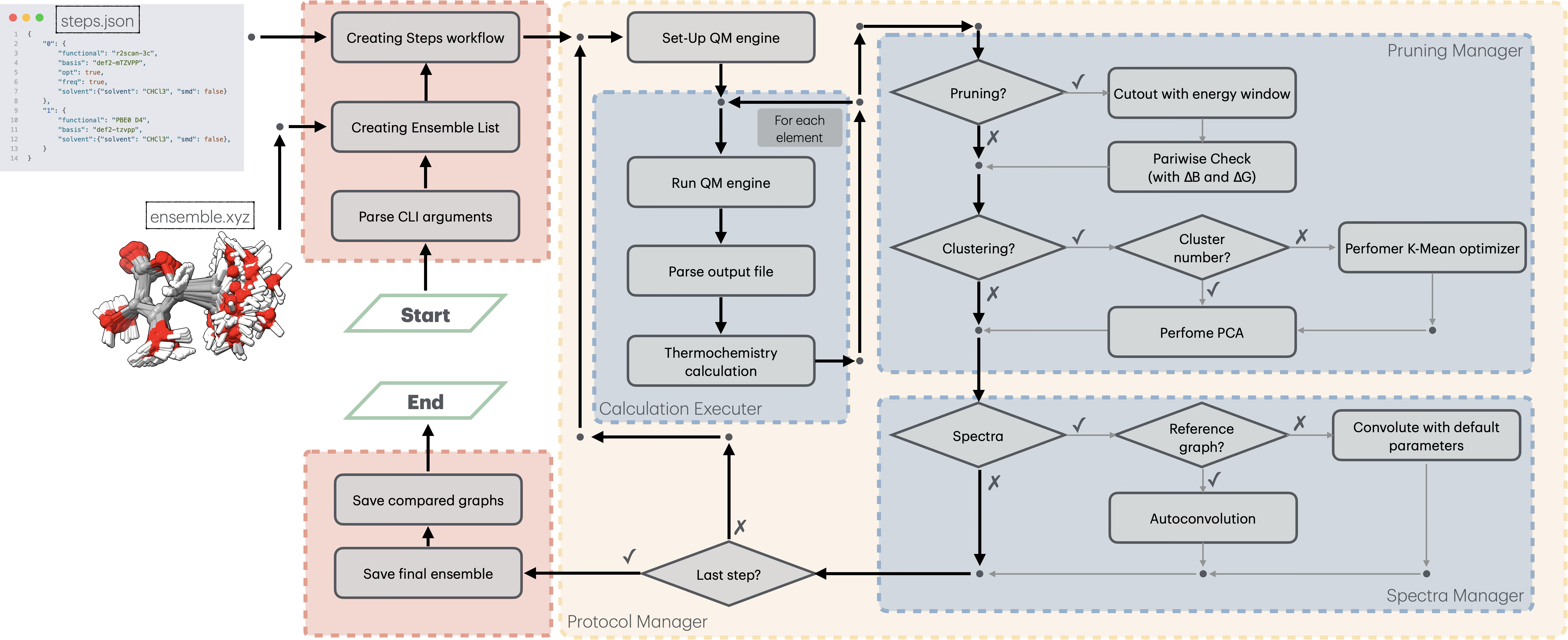
Analysis Workflow
This guide details the internal workflow of Ensemble Analyzer, illustrating how data flow from the initial input through the refinement pipeline to the final property generation.
1. Input & Initialization
The workflow begins by parsing the command-line arguments and initializing the core managers.
1.1 Data Loading
The launch.py entry point triggers the loading phase:
Ensemble Loading: The geometry file (e.g.,
.xyz) is parsed into a list ofConformerobjects.Protocol Loading: The JSON protocol is deserialized into a list of
Protocolobjects, defining the sequence of computational steps (e.g., Optimization \(\to\) Frequency \(\to\) Single Point).Configuration: Global settings (temperature, CPU count, solvent models) are loaded into the
CalculationConfigobject.
1.2 Initial Analysis
Before starting the refinement loop, if the ensemble contains sufficient structures (\(N > 30\)), an initial Principal Component Analysis (PCA) is performed on the input geometries to visualize the starting conformational space coverage.
2. The Refinement Loop
The core logic is handled by the CalculationOrchestrator, which iterates through each step defined in the protocol.json. For each protocol step, the ProtocolExecutor performs the following operations:
2.1 Quantum Mechanical Calculations
For every active conformer that has not yet been calculated at the current level:
Input Generation: The
CalculationExecutorgenerates input files for the external QM engine (ORCA or Gaussian).Execution: The calculation is run (Optimization, Frequency, or Single Point).
Parsing: Results (Energy, Geometry, Dipoles, Rotational Constants, Vibrational Frequencies) are parsed and stored in the
EnergyStoreof the conformer.Checkpointing: The
CheckpointManagersaves the state atomically after every calculation to prevent data loss.
2.2 Pruning Stage
After the calculation phase, the PruningManager filters the ensemble to remove high-energy structures and geometrically redundant conformers. This step is critical to reduce computational cost for subsequent, more expensive steps.
The pruning logic consists of two main filters:
Energy Window Filtering: Conformers with a relative energy above the threshold (\(\Delta E > \text{thr}G_\text{max}\)) are immediately deactivated.
Parameter:
thrGMAX(defined inthreshold.jsonor protocol).
Geometric Filtering (Duplicate Removal): Instead of computationally expensive RMSD alignments, EnAn uses Rotational Constants (\(B\)) and Electronic Energy (\(E\)) as descriptors to identify duplicates. Two conformers \(i\) and \(j\) are considered identical if: $\(|\Delta E_{ij}| < \text{thrG} \quad \land \quad |\Delta B_{ij}| < \text{thrB}\)$
Parameters:
thrG(Energy tolerance),thrB(Rotational constant tolerance).Validation: For logged duplicates, an RMSD based on the Euclidean Distance Matrix (EDM) eigenvalues is calculated for verification.
Note: Pruning can be disabled for specific steps by setting
"no_prune": truein the protocol.
2.3 Clustering & Analysis
If clustering is enabled in the protocol ("cluster": true or specific integer), the ClusteringManager performs an unsupervised structural analysis to group conformers and optionally reduce the ensemble.
The workflow utilizes invariant features to avoid coordinate alignment issues:
Feature Extraction: The eigenvalues of the Euclidean Distance Matrix (EDM) are computed for each conformer. These are invariant to translation and rotation.
PCA (Principal Component Analysis): Dimensionality reduction is applied to the EDM eigenvalues.
K-Means Clustering:
If a specific number of clusters is provided, K-Means is run directly.
If set to
auto, the optimal number of clusters (\(k\)) is determined via Silhouette Score analysis (scanning \(k=2\) to \(k=N_{conf} \times 0.8\)).
Ensemble Reduction: The ensemble is reduced by retaining only the representative conformer (lowest energy) from each cluster.
2.4 Spectral Generation
The final stage of a protocol step involves generating continuous spectra from discrete transitions. This is handled by the graph module.
Vibronic Spectra (IR, VCD): Convolved using Lorentzian functions.
Electronic Spectra (UV-Vis, ECD): Convolved using Gaussian functions.
Population Weighting: All spectra are weighted based on the Boltzmann population of the conformers, calculated using the relative Gibbs Free Energy (\(\Delta G\)) at the specified temperature (\(T\)).
3. Finalization & Output
Once all protocol steps are completed, the CalculationOrchestrator finalizes the workflow:
3.1 Data Export
final_ensemble.xyz: A multi-structure XYZ file containing all surviving conformers, sorted by energy.checkpoint.json: A complete state file allowing for restarts or post-processing analysis.
3.2 Comparative Plotting
The plot_comparative_graphs module automatically generates overlay plots (e.g., IR_comparison.png, UV_comparison.png). These plots visualize the evolution of the computed spectra across the different protocol levels (e.g., comparing the spectrum after SP vs OPT+FREQ), allowing for quick assessment of convergence and method dependence.
3.3 Reporting
A summary table is printed to the log (output.out), detailing:
Final energies (E, H, G) and ZPVE.
Boltzmann populations.
Total elapsed time and final retention rate.